Testing The Model

Our central idea is that market price formation is driven by sums of logarithmic returns of many transactions.  We believe that the price formation process of the continuous double auction has heavy tails.  Over times as short as a minute, the returns begin to converge to a stable distribution by the generalized central limit theorem.  When we try to fit long stretches of returns over many days, we quickly find that the data do not conform to a stationary stable distribution.  The tails of the return data are too light.  We either have the wrong distribution or bad methods.  By experimentation we find that the method of maximum likelihood fitting of the distribution shape parameter, α, can be significantly affected by contamination with an excess of returns in the middle of the distribution.  This distorts the calculation of α, even though the tails of the contaminated data are not changed.  When we look at events that are in the process of converging to a stable regime, by a two tailed continuous double auction model, we find that there are initially an excess of zero returns in the model, upon summation these disappear, but to the extent that a sample has not fully converged to a stable regime, an excess of small returns artificially lowers α.

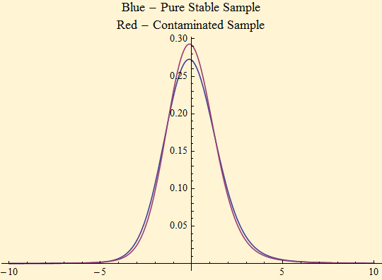
The experiment below shows a stable random sample generated with parameters: {1.8, 0.2, 1,0 }. It is fit by the maximum likelihood method below.

Stable Parameters {α, β, γ, δ} = {1.80643, 0.535578, 1.03628, 0.0723559}

The sample is contaminated with a hundred uniform random variables range {-0.2, 0.2} and refit.  The graph below shows the plot of the density of the two fits.  Calculated α is lower in the sample with extra mass added to the center of the distribution, even though the mass on the tails has not changed.

Stable Parameters {α, β, γ, δ} = {1.77813, 0.438959, 0.965275, 0.0620158}

In high resolution minute by minute data, this phenomenon may be contributing because the sums of log returns have not fully converged to a stable regime.  We believe, there is more to the problem, namely that the scale factor, γ, of the distribution is changing on a minute by minute basis.  The ultimate collection of returns we see is derived from a mixture of stable distributions with varying γ.  The variation of the scale parameter, γ, is not random, but shows serial dependence with an interesting pattern.  The blue curve is the autocorrelation function of the raw absolute value of the log returns.  Our data set consists of 391 returns a day minute by minute.  It does not include the pre-market or after-market trading.  The log return from the previous close to the open is included as the first return of the day and all the days are concatenated.  The spikes are caused by the inter-day returns, but there is an intra-day pattern that is caused by higher volatility at the begin and end of the day.  From day to day there is serial dependence that slowly decays.  Fifteen days of data are shown in the graph.  The red graph divides each day's returns by the scale factor for that day.  There is no attempt to correct the cyclic intra-day variation.  With this maneuver, most of the day to day serial dependence disappears, but the intra-day cycle and inter-day spikes remain.

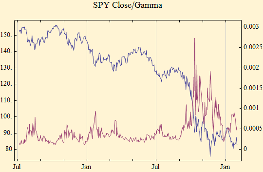
The next graph shows the plot of the SPY ETF closing price in blue and the daily stable γ, calculated since July 2007.  The spike in volatility at the end of the series is dramatic and historical.  There has not been such a spike in the history of the SPY ETF and a look at other historical data such as the Dow Jones Industrial Average, suggests this level of volatility has not occurred since the 1930s.  As this page is updated, it will be interesting to see how this plays out.  Right now it presents an opportunity to test our model.  Note that spikes of volatility (γ) are associated with price declines.  Periods of falling volatility are associated with rising prices.

Our hope is that our relatively simple model of varying scale factor will have a relatively constant shape parameter, α.  Such a finding would make analysis of the problem somewhat mathematically tractable.  We expect the β parameter to vary on a minute to minute basis dependent upon the ratio of orders filled in the buy and sell order books.  On a minute to minute basis, δ should be essentially 0.

Mean stable parameters { 1.82031, -0.0375413,  0.000477175, -0.00000580621}

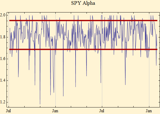
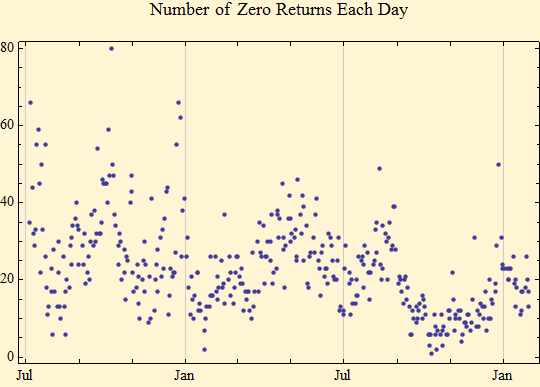
The graph above is the calculated value of α for each day of the sample.  The heavy red lines are the 95% confidence intervals based on the mean α and a sample size for each day of 391.  Some days are actually shorter because of early market closing before holidays.  There are more excursions outside the confidence intervals than we would predict, but it is encouraging that most of the time α is close to the mean, especially at the end of the series where we have begun to experience extreme volatility.  The scale factor is changing, but the basic fractal dimension, α, of the market behavior seems to be rather constant.  Some of the variation and low values for α calculated may have been from excess zero returns in the sample.  Note that there are fewer zero returns at the end of the series when volatility and market volume were high, suggesting more complete convergence to a stable regime at the one minute time interval.

We can use extreme value distributions and theory to make an estimate of α from the tail data, thereby overcoming some of the problem of too much mass in the middle of the mixture sample of our data.  The idea here is that tail events occur with some regularity.  So we have selected the maximum values from each day's morning and afternoon events and fit this distribution to a generalized extreme value distribution (gev).  The ξ parameter of the gev is equivalent to 1/α of a stable distribution from which it is derived; thus we have another method of calculating α.

Before September 2008, this calculation worked well for the whole database, with the surge of volatility since then the magnititude extreme events in the last part of the data set overwhelms the calculculation.  We believe the distribution of the intra-day gamma has significantly changed.  This calculation is now being performed on the last part of the data that begins with September 2008.

Sample size of right tail 210.

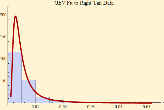
Calculated stable α 1.9203.

Sample size of left tail 210.

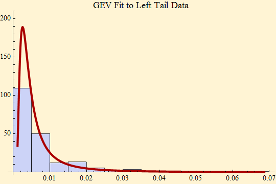
Calculated stable α 1.57121.

At this point with a smaller data set the tails are different.  We expect that as we accumulate more data at the current volatility levels they will become closer.  Before the market volatility in September 2008, these fits seemed more consistent with a stationary α at approximately 1.8.  

When we fit the whole raw data set, we get the following result, with the finding of an artificially very low α.  The scaled data find an α more consistent with the daily fits, but now the γ and δ are scaled to γ = 1.

Stable fit to raw data {α, β, γ, δ} = { 1.38814,  0.00000000280358,  0.000367778, -0.0000000972526}

Stable fit to scaled data {α, β, γ, δ} = { 1.79855,  0.00000000988973,  1.01309,  0.000111789}

We now analyze the properties of the scale factor, γ, which is a measure of market volatility.  The graph below shows the plot of γ, calculated by two methods one is a quick method based on the stable characteristic function the other is by the maximum likelihood method--the results are virtually identical.

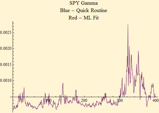
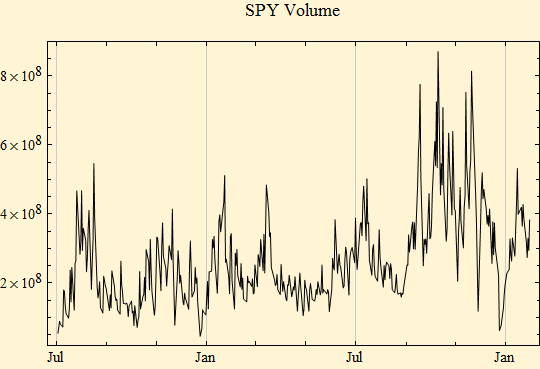
The pattern of volatility is related to market volume, but they are not directly proportional .  The following plot shows the daily volume over the same time interval as the sample.

We show below the histogram of the daily γ data beginning September 2008.  These data are clearly not random.  The idea of showing their histogram and a fit to a lognormal distribution is mainly to show that the data are somewhat constrained.  Until the most recent week, the sample was well fit by the lognormal distribution, but the extreme results of the recent week are too heavy to be consistent with the rest of the sample and a lognormal fit.  (The data before September 2008, were also fit with a log normal distribution, but the parameters have changed, so we are tracking the more recent data set.)

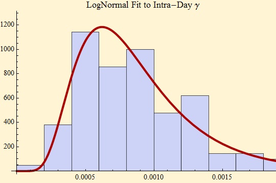
MLE fit to lognormal distribution, loglikelihood and parmeters
{678.354, {μ -> -7.15085, σ -> 0.482587}}

The Q-Q plot is shown.  The lognormal fit was quite good until the current weeks, when the divergence of the tail began with the current high volatility.  We are likely in a new era of volatility which will persist for some time.  The intra-day scale factor may not be sufficiently constrained to fit to a model such as a lognormally scaled stable distribution.

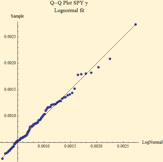
We are quite pleased with the performance of the model over this very extreme market period, but the constraint of a lognormal distribution for the scale factor seems to have different parameters since September 2008.  We will update this page periodically.  This model simply is a non-stationary stable distribution with a varying scale factor or amplitude.  Since stable distributions can have heavy tails they are prone to extreme jumps.  The varying scale factor is multiplicative so the jumps can be magnified greatly. Over the last year we have seen this scaling increase by a factor of 13.  The scaling always in the past has shown serially dependence, so the current volatility is not likely to disappear soon.  By this model extreme events are common when volatility is high and crashes should be expected.

© Copyright 2009 mathestate    Sun 1 Feb 2009